How to Add a Search Box to a Slicer to Quickly Filter Pivot Tables and Charts

Bottom line: Learn how to add a search box to a slicer to quickly filter your pivot tables, pivot charts, or Excel Tables.  Includes a video tutorial that explains the setup in detail.

Skill level: Intermediate

Video Tutorial: How to Add a Search Box to a Slicer

Watch video on YouTube (and hit the Like button!)

Download the File

Download the file to follow along.

Add A Search Box To A Slicer.xlsx (278.7 KB)

Problem: It’s Hard to Navigate Slicers with Lots of Items!

Kati asked a great question about adding a search box to a slicer.  She has a slicer with over 200 items (names) in it, and it takes a lot of time to scroll horizontally through the slicer to find a name.

How Can We Add a Search Box to the Slicer?

Unfortunately there is no built-in way to add a search box to a slicer in Excel.  So this solution is a bit of a workaround.

The good news is that it does NOT require any macros or coding.  This solution uses the filter drop-down menu in another connected pivot table, and it is pretty easy to implement.

Note: The filter search box was introduced in Excel 2010 for Windows, so this solution will work in the 2010, 2013, or 2016 versions for Windows.  The solution will also work for the Mac 2016 version of Excel.

Step-by-Step Instructions

The video above explains how to add the search box to the slicer.  Here are the basic steps that I explain in the video.

1. Insert a slicer on the worksheet.
2. Make a copy of the pivot table and paste it next to the existing pivot table.
3. The new pivot table will also be connected to the slicer.  The slicer is connected to both pivot tables.
4. Remove all fields from the areas of the new pivot table.
5. Add the slicer field to the Filters area of the new pivot table.
6. Move the slicer on top of the cell that contains the filter drop-down button in the Filters area of the new pivot table.
7. Adjust the column width so the filter button is just to the right of the slicer.
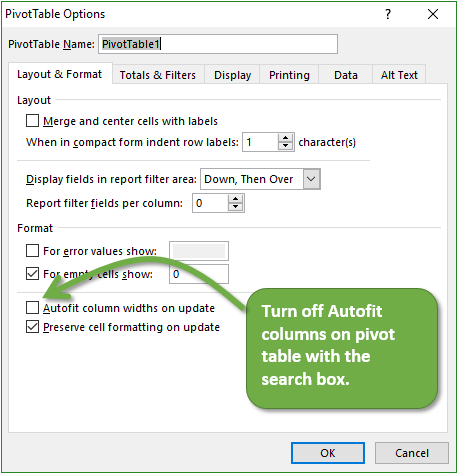
8. Turn off the Autofit column widths option on the new pivot table. (Right-click pivot table > PivotTable Options…)
   
9. Hide the column that contains the field name in the Filters area of the new pivot table.

Now you should be able to click the filter drop-down button and use the Search box to quickly find items in the field (slicer) and apply filters.

Keyboard Shortcuts

In the video I mention that you can press the letter “e” on the keyboard to place the text cursor in the search box.

Checkout my article on 7 Keyboard Shortcuts for the Filter Drop Down Menus for more shortcuts for this menu.

You can also add a Hyperlink to the cell that contains the Filter Button.  Then press Alt+Down Arrow to open the menu and jump the cursor into the search box.

Those shortcuts will make it really fast to get to the search box to filter the slicer.  The hyperlink text also alerts your users that there is a search box available for the slicer.

Use the Slicer Search Boxes on Multiple Slicers in Dashboards

The slicer search boxes are great for dashboards and pivot charts too.  You can repeat the process to setup search boxes for all the slicers in your dashboard.

Click to Enlarge

Checkout my free video series on pivot tables and dashboards to learn how to use pivot tables to create the dashboard in the image above.  It’s easier than you think!

Will You Add Slicer Search Boxes to Your Pivot Tables and Charts?

Please leave a comment below with any questions or suggestions.

The post How to Add a Search Box to a Slicer to Quickly Filter Pivot Tables and Charts appeared first on Excel Campus.