Bottom Line: Learn an easy way to calculate running totals in Excel Tables, and how to calculate running totals based on a condition or criteria.
Skill Level: Intermediate
Video Tutorial
Download the Excel File
You can download the Excel file to follow along and practice writing your own formulas for running totals.
![]() Running Totals In Excel Tables - 3 Methods.xlsx (174.7 KB)
Running Totals In Excel Tables - 3 Methods.xlsx (174.7 KB)
Running Totals in Excel Tables
Paul, a member of our Elevate Excel Training Program, posted a great question in the Community Forum. He wanted to know the best way to create running totals in Excel Tables, since there are multiple ways to go about it.

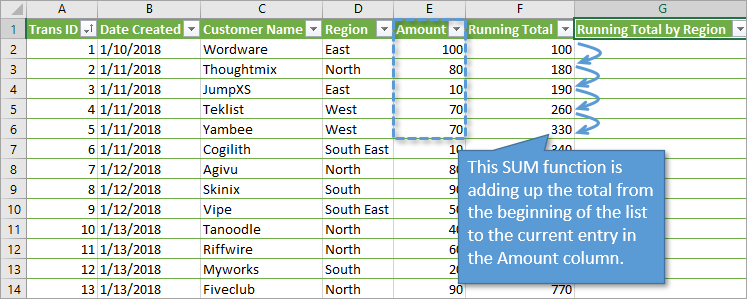
The running total calculation sums all of the values in a column from the current row the formula is in to the first row in the data set.
Therefore, we need to create a range reference that always starts at the first row in the column, down to the current row the formula is in.
When using Excel Tables, it's best to use structured references (references to the table and column names) for running totals. Using regular cell references like ($A$2:A3) can cause errors in your formulas, more on that below.
Unfortunately, there is no straightforward way to create this reference with Table formulas. There are still many ways to solve this problem and I'll share three methods in this post.
Method #1: Reference the Header Cell
My preferred method is to reference the header cell to create the absolute reference for the first cell in the range. Then reference the cell in the row that the formula is in for the last cell in the range. Here is an example.
=SUM(tblSales[[#Headers],[Amount]]:[@Amount]])

The reason I reference the header cell (tblSales[[#Headers],[Amount]]) is because the reference will NOT change as the formula is copied down. This makes it an absolute reference.
The ending reference [@Amount] creates a relative reference to the row that the formula is in.
In everyday terms, you've just told Excel to add up everything from the beginning of the Amount column (including the header row) down to the row the formula is in, and to return that value in the Running Total column.
Because we are using an Excel Table, the formula will automatically be copied down the entire column. You can see how each cell adds the current amount to the existing total to give a running total.
Tips for Writing the Formula
- When writing this formula you can click the header cell to create the reference (tblSales[[#Headers],[Amount]]). You do NOT have to type out the entire reference.
- After clicking the header cell, click into the end of the formula to edit it and type a : colon. Then select the cell in the row the formula is in to create the ending reference [@Amount].
A Few Notes About the References
There are a few good things to know about this running total formula with structured references.
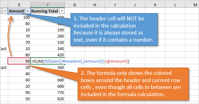
- The header cell always contains the text data type. Therefore, the value in the header cell is NOT included in the SUM formula calculation. Even if the header cell contains a number, that number is stored as text and will not be included in the calculation.
- When looking at the formula in Edit mode, only the cells in the header row and current row are selected. Excel does put a colored border around the entire range. This does not impact the results of the formula. All of the cells between the header cell and current row are included in the calculation. It is just a visual nuance to be aware of.
Why Use Structured References?
You may be wondering why I use structured references (tblSales[[#Headers],[Amount]]:[@Amount]]) instead of regular range references ($A$2:A2) in the SUM formula.
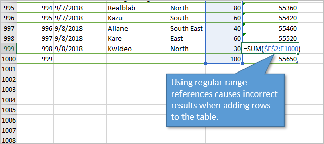
A formula with regular range references is probably easier to create and read in this scenario. However, the formulas don't always get copied down properly. If you add new rows to the bottom of the table, the running total formula will not create a relative reference to the row the formula is in. Instead, it will likely keep a reference to the last row in the table BEFORE rows were added. This leaves us with incorrect results.
This happens because Excel remembers ONE formula for the entire column and copies it down. When using structured references, the formula text is the SAME in every cell of the running total column. Every cell contains: =SUM(tblSales[[#Headers],[Amount]]:[@Amount]])
Method #2: Mixed References
Another option is to create an absolute reference to the first cell in the column, combined with a structured reference for the last cell.
=SUM($E$2:[@Amount])
This method seems to work as well as the referencing the header row. I believe I've had issues with it in older versions of Excel, but can't seem to break it in the current version of Microsoft 365. Therefore, my preference is to use full structured references.
Please leave a comment below if you use this method and/or have issues with it.
Method #3: SUM & INDEX
Another popular alternative uses the INDEX function within SUM.
=SUM(INDEX([Amount],1):[@Amount])
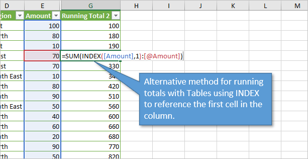
The INDEX function is used to create a reference to the first cell in the column because we reference a 1 for the row_num argument. INDEX([Amount],1)
This method works just as well, but there are two drawbacks that make me not love it as much:
- The formula is more difficult to read and understand for users of your file that are not familiar with the INDEX function.
- The entire column is referenced in the array argument of INDEX. This creates a colored border around the entire column when in formula edit mode, even though the function evaluates to create a reference to just the first cell. To me, this is a bit more confusing than the reference the to first and current cells that the first method uses.
Which Method is Best?
Honestly, none of these solutions are perfect. Each has their pros & cons. I just find method #1 easier to read, write, and understand.
It would be great if structured references had a better way to reference other cells in the column like the first cell, last cell, cell above, cell below, etc. I know we can create these with nested functions, but it makes it more challenging for other users of our files to understand.
Running Total with Conditions
We can also use these any of these running range references in the SUMIF(S) function to create running totals based on a condition or criteria. In this example I create a running total by region. Here is an example of the formula.
=SUMIF(tblSales[[#Headers],[Region]]:[@Region],[@Region],tblSales[[#Headers],[Amount]]:[@Amount])
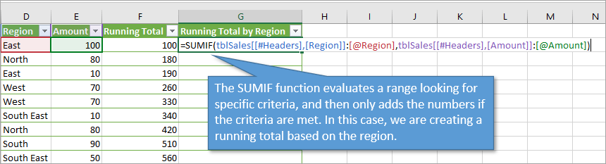
Here is an explanation of each component of the formula:
- The first argument in SUMIF is the range we want to evaluate (tblSales[[#Headers],[Region]]:[@Region]). This uses the same running range reference method.
- The second argument is the criteria or condition that we want to filter the range for ([@Region]). This is the value in the same row the formula is in from the Region column.
- The third argument is the sum range which contains the values we want to sum with the criteria is True (tblSales[[#Headers],[Amount]]:[@Amount]).
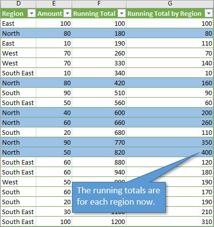
Now the running total column reflects running totals for each region. I've highlighted one of the regions (North) in the image below so you can see how the running totals are region-specific.
Conclusion
The running total is especially useful if we are making additions to the list over time and want to track our progression. Using structured references in the formula prevents errors when adding new rows to the table.
Unfortunately, there isn't a straightforward way to create the running range reference with table formulas. The three methods presented in this post should help you create the formulas. I prefer method #1, but it's good to know them all since you will probably come across them in your Excel journey.
The running range reference can also be used with other functions like AVERAGE, AVERAGEIFS, COUNT, COUNTIFS, MIN, MINIFS, MAX, MAXIFS, etc. to calculate different running metrics.
Please let us know if you have any questions, suggestions, or alternative methods in the comments below.
The post 3 Ways to Calculate Running Totals in Excel Tables + By Condition appeared first on Excel Campus.


